The Universe conspired to bring me precompiled binaries for Idris

Installing it with cabal on Windows proved impossible. A SuSe VM on VirtualBox couldn’t cut it either. Actually installing MinGW, which was the recommended way on WIndows, didn’t give me Idris, either. But still, I wanted it. And, sure enough, as Paulo Coelho predicted, the Universe conspired to help me get it, and one can now download precompiled binaries for Windows!

Now that I had a real dependently-typed programming language, with realistic-looking tutorials and documentation, I thought it was a great excuse to implement type-safe dimensional calculations in it. The resulting code is so terse, compared to the Scala example, it almost feels like cheating. In the beginning, is the dependent type itself.

data DimVal : Int -> Int -> Int -> Int -> Type where
    DV :  (m:Int) -> (k:Int) -> (s:Int) -> (a:Int) -> (v:Float) -> DimVal m k s a

Please compare it with the Scala (and C++) equivalent. The similarities are obvious but this version completely blends the two levels together. DimVal is a type constructor indexed by four integers and DV is its sole constructor.

Calculating with these types needs the usual arithmetic operations. Unfortunately, trying to overload the operators did not work for me, as they were imported already by the Num class in the Prelude.

||| The Num class defines basic numerical arithmetic.
class Num a where
(+) : a -> a -> a
(-) : a -> a -> a
(*) : a -> a -> a
||| Absolute value
abs : a -> a
||| Conversion from Integer.
fromInteger : Integer -> a

DimVal cannot be made an instance of Num, because types need to be closed under all three operations, and this cannot be the case, since the point is to represent each dimension vector by a different type. So I faked four appropriate operators.

infixr 10 /+/
(/+/) : DimVal m k s a -> DimVal m k s a -> DimVal m k s a
(DV m k s a v1) /+/ (DV m k s a v2) = DV m k s a (v1+v2)

infixr 10 /-/
(/-/) : DimVal m k s a -> DimVal m k s a -> DimVal m k s a
(DV m k s a v1) /-/ (DV m k s a v2) = DV m k s a (v1-v2)

infixr 20 /*/
(/*/) : DimVal m1 k1 s1 a1 -> DimVal m2 k2 s2 a2 -> DimVal (m1+m2) (k1+k2) (s1+s2) (a1+a2)
(DV m1 k1 s1 a1 v1) /*/ (DV m2 k2 s2 a2 v2) = DV (m1+m2) (k1+k2) (s1+s2) (a1+a2) (v1*v2)

infixr 20 ///
(///) : DimVal m1 k1 s1 a1 -> DimVal m2 k2 s2 a2 -> DimVal (m1-m2) (k1-k2) (s1-s2) (a1-a2)
(DV m1 k1 s1 a1 v1) /// (DV m2 k2 s2 a2 v2) = DV (m1-m2) (k1-k2) (s1-s2) (a1-a2) (v1/v2)

Next up, printing dimensioned values. For this, I used an intermediate Dimension type.

data Dimension : Type where
    Dim : (m:Int) -> (k:Int) -> (s:Int) -> (a:Int) -> Dimension    

unitToStr : Dimension -> String
unitToStr (Dim m k s a) =
    case (m, k, s, a) of
        (0,0,1,1) => "C"
        (1,1,-2,0) => "N"
        (0,0,-1,0) => "Hz"
        (-1,1,-2,0) => "Pa"
        (2,1,-3,-2) => "ohm"
        (2,1,-3,-1) => "V"
        (-2,-1,3,2) => "S"
        (2,1,-3,0) => "W"
        (2,1,-2,0) => "J"
        (-2,-1,4,2) => "F"
        (2,1,-2,-2) => "H"
        (2,1,-2,-1) => "Wb"
        (0,1,-2,-1) => "T"
        _ => (if m /= 0 then "m" ++ (if m /= 1 then (show m) else "") else "") ++
            (if (m /= 0) && (k /= 0) then "." else "") ++
            (if k /= 0 then "Kg" ++ (if k /= 1 then (show k) else "") else "") ++
            (if (abs(m) + abs(k)) /= 0 && s /= 0 then "." else "") ++
            (if s /= 0 then "s" ++ (if s /= 1 then (show s) else "") else "") ++
            (if (abs(m) + abs(k) + abs(s)) /= 0 && a /= 0 then "." else "") ++
            (if a /= 0 then "A" ++ (if a /= 1 then (show a) else "") else "")
            
toStr : DimVal m k s a -> String
toStr (DV m k s a v) = (show v) ++ " " ++ (unitToStr (Dim m k s a))
    
instance Show (DimVal m k s a) where
    show dv = toStr dv

The Num class was out of the question, but Eq and Ord are readily instantiable.

dimValEq : DimVal m k s a -> DimVal m k s a -> Bool
dimValEq (DV m k s a v1) (DV m k s a v2) = (v1==v2)
    
dimValComp : DimVal m k s a -> DimVal m k s a -> Ordering
dimValComp (DV m k s a v1) (DV m k s a v2) = compare v1 v2

instance Eq (DimVal m k s a) where
    dv1 == dv2 = dimValEq dv1 dv2

instance Ord (DimVal m k s a) where
    compare dv1 dv2 = dimValComp dv1 dv2

Idris has syntax support for creating DSLs so, a native Idris speaker would probably go on to create a better DSL for creating values, arithmetic etc. I’ll just show how type-safe calculations can naturally be encoded in plain Idris. I did not go into the trouble of defining all named physical types but I guess you see how this can be done without any problem.

Mass : Type
Mass = DimVal 1 0 0 0

mass : Float -> Mass
mass = DV 1 0 0 0

main : IO ()
main = 
    let x = DV 1 1 (-2) 0 14.5 in
    let y = DV 1 1 (-2) 0 15.5 in
    let z = DV 2 2 0 0 15.5 in
    let xpy = x /+/ y in
    let xmy = x /-/ y in
    let xtz = x /*/ z in
    let xdz = x /// z in
    let m : Mass = mass 12.6 in
        do
            putStrLn (show m)
            putStrLn (show x)
            putStrLn (show y)
            putStrLn (show z)
            putStrLn (show (x == x))
            putStrLn (show (x == y))
--            putStrLn ((show (y == z))) -- Doesn't even compile!
            putStrLn (show (x < y))
--            putStrLn ((show (z < y))) -- Doesn't even compile!
            putStrLn (show xtz)
            putStrLn (show xdz)

It does feel like cheating, doesn’t it? Calculating with physical types is actually done at two levels: the values themselves are operated upon as if they were dimensionless, while the dimensions are vectors representing exponents and are operated upon using exponent arithmetic. Idris handles both levels in the same way, very naturally. It is said that all high-level languages are equivalent in the computations they can express, but their compilers are certainly not equivalent.

My Frugal Summer of Code, part 2

Here I am, continuing my foray into the realm of array programming, that started in my previous post. Let me start with a disclaimer: I do not claim that what you read here is good, idiomatic J.This is not a J tutorial. I mean it as an exposé of the notions of array programming and how they can enhance the worldview of the traditional programmer. I’d love it if it could also be a bridge between mainstream FP and Array Programming, but I’m afraid I’m not sufficiently proficient in either to do it.

Remember the last five lines of code? I’m going to dissect them now for your benefit.

NB. Locations (mask bits) where digits have lines 
digitmasks =. '         ' ~:"(1) (,"2 digits)

Laid out, this means: concatenate all lines in each digit (keeping them in three lines serves only for displaying them). This is done by , (called append), applied to cells of digits of rank 2 (the "2 modifier, called an conjunction in J). Then, compare lines (cells of rank 1, the "1 thing) of that, using the “not equals” comparator (the ~:) to a literal with 9 spaces.

This gives you a bit (an 1) whenever there’s anything than a space. I can do that because the digits, as defined, when they share a graphic element, it’s always the same in the same location. So I’m getting rid of some excessive information to make my life easier. So, digitmasks is the following.

0 1 0 1 0 1 1 1 1
0 0 0 0 0 1 0 0 1
0 1 0 0 1 1 1 1 0
0 1 0 0 1 1 0 1 1
0 0 0 1 1 1 0 0 1
0 1 0 1 1 0 0 1 1
0 1 0 1 1 0 1 1 1
0 1 0 0 0 1 0 0 1
0 1 0 1 1 1 1 1 1
0 1 0 1 1 1 0 1 1

NB. Locations where digits share mask bits
maskcompmatrix =. (-"1/~ digitmasks) ="0 ] 0

Moving on, first, I make a table where, I subtract each line (i.e. digit bitmask) from each other. The -"1/~ digitmasks thing is shorthand for digitmasks -"1/ digitmasks, i.e. tabulate (the / adverb – another kind of higher-level construct, like conjunctions – for a dyadic operation) the operation “subtract each line” (the -"1). Afterwards, the whole thing is compared, bit by bit (the ="0) to zero. The result is a 10 x 10 x 9 bitmask array. Are you getting the hang of it?

NB. Count of similar mask bits between digits
diffmatrix =. +/"1 maskcompmatrix

Further, I sum: insert, using the / adverb, the operation “plus” (the + verb) at the level of each line (the "1 conjunction) on maskcompmatrix. This gives a 10 x 10 array of the number of same bits in each bitmask (digit).

9 5 6 6 5 6 7 6 8 7
5 9 4 6 7 4 3 8 4 5
6 4 9 7 4 5 6 5 7 6
6 6 7 9 6 7 6 7 7 8
5 7 4 6 9 6 5 6 6 7
6 4 5 7 6 9 8 5 7 8
7 3 6 6 5 8 9 4 8 7
6 8 5 7 6 5 4 9 5 6
8 4 7 7 6 7 8 5 9 8
7 5 6 8 7 8 7 6 8 9

Now comes the easy part.

NB. Outside the diagonal: Digits that share 8 out of 9 mask bits
offbyone =. diffmatrix ="(0) 8

I make a 10 x 10 array of selectors (bits) when digits share 8 out of 9 bits.

offbyones =. (monad : '< y # i. 10')"1 offbyone

Then, I make a vector (list, in J) of which digits share 8 bits for each digit.

┌─┬─┬┬─┬┬───┬───┬─┬─────┬─────┐
│8│7││9││6 9│5 8│1│0 6 9│3 5 8│
└─┴─┴┴─┴┴───┴───┴─┴─────┴─────┘

I wanted to spare you (and me!) the trouble of bringing up “boxing” but, since the shape is irregular, it was really the easiest solution. Boxing (conveniently displayed with actual boxes) creates an atomic value of anything you put into it.

And, in reality, I found out that it makes calculations simpler if the digits themselves are included, so I really need the following.

NB. Digits that share 8 or 9 (i.e. themselves) mask bits
sameandoffbyone =. diffmatrix >:"(0) 8

sameandoffbyones =. (monad : '< y # i. 10')"1 sameandoffbyone

┌───┬───┬─┬───┬─┬─────┬─────┬───┬───────┬───────┐
│0 8│1 7│2│3 9│4│5 6 9│5 6 8│1 7│0 6 8 9│3 5 8 9│
└───┴───┴─┴───┴─┴─────┴─────┴───┴───────┴───────┘

This was sort of easy, wasn’t it? I’m afraid the rest will be a little more complicated. I’ll throw it all in one glob, and focus on the big picture first. The operation I’m trying to achieve, is fix broken account numbers by trying similar digits, where similar is defined by off-by-one bit.

NB. fold operation to produce the combinations
foldop =. dyad : ',/ <"1 (>y) ,"1/ (,. >x)'
identity =. <''

NB. Use if checksum is <> 0: try combinations with digits off by one mask bit and see which (if any) produce checksum of 0
alternatives =. monad define
 alt =. >"0 foldop/ identity ,~ |. y { sameandoffbyones
 ((checksum"1 = 0:) alt) # alt
)

There’s a fold taking place, which is a common thing in FP. The first complication is that, in J, for reasons of uniformity with its right-to-left evaluation order, when you fold a list (remember, a list is a vector of something) you also do it right-to-left. That’s why I reverse (the |. thing) the result of indexing (the {) sameandoffbyones by the account digits (y stands for the argument in a monadic verb). Then I append the identity element, which is a boxed empty list. Folding takes place, and I’ll explain the operation folded next but, for now, let’s stick to what the fold produces, which is a list of boxed candidate account numbers, which are unboxed (the >"0) and then checked with checksum (the checksum"1 = 0: is actually a composite verb!) and only those with zero checksum are kept (operation copy, the #).

Example usage:

alternatives 2 4 4 4 1 2 5 6 7

2 4 4 4 1 2 5 6 1
2 4 4 4 1 2 9 8 7
2 4 4 4 7 2 6 6 1

However, don’t try it on 7 2 3 4 5 6 7 8 9. It produces 109 possible alternatives! In retrospect, this error correction policy is not very robust or, rather, the checksum used in not suitable to how digits can be misread.

Let’s go back to the folded operation now. I won’t go into it symbol-by-symbol but here’s an English description. One operand holds a list of boxes with partial account numbers, and the result is also a list of boxes with longer partial account numbers, formed by appending the initial partial account numbers with all alternatives for the current digit, held by the other operand as a boxed list.

Have I picked your curiosity until now? Have I succeeded in presenting J as more than a curiosity itself? There is real power in its notions and it goes beyond its conciseness. Imagine all these operations using standard Scala, for example. “It’s easy if you try.” I think it is a useful thing to add to standard FP, which lacks the language to talk about arrays at the level that array programming languages do. I have not even found a data type to represent arbitrary-ranked arrays, let alone how to represent ranked operations and implicit loops and stuff. But I think it can be done, and I’m setting it as a wanna-do-it for the future.

My Frugal Summer of Code

The title being a wordplay on “Google Summer of Code” does not mean that it is not entirely true, as there is hardly any time during vacationing with two little children to write much code. And I admit that most of what you’ll see in this post was written pre- and post-vacations. But I did read a lot of stuff on array programming, APL, J, papers on array functional programming. I thought really hard (but vacation-grade hard) about how some of these things can be grafted on a more conventional functional language. And I did make an honest effort to find a Java or Scala library for dense multidimensional arrays that could provide a basic substrate for such an effort. If the job, Flying Donut or life, in general, let me, you’ll hear more in another post.

The current post, however, will use J to tackle a code kata I found, which I thought would be ideal for some array-fu.

Assume you have the three lines that constitute an account number. The first thing you should do is separate the nine “digits”. Conveniently, the same functionality can be used to generate some data useful in the sequel, so let’s start by separating the ten digits 0 – 9.

alldigits =. ] ;._2 (0 : 0)
 _     _  _     _  _  _  _  _
| |  | _| _||_||_ |_   ||_||_|
|_|  ||_  _|  | _||_|  ||_| _|
)

NB. Break in 3x3 cells
chop =. monad : ',/ (3 3 ,: 3 3) ];._3 y'

digits =. chop alldigits

I know, most of it looks like a cartoon character swearing. What you see in the above is a handy way of writing multi-line data and a handy higher-level operation to apply an operation to subarrays of an operand. Let’s chop a sample account number.

NB. A number with no wrong digits
num =. ] ;._2 (0 : 0)
    _  _     _  _  _  _  _ 
  | _| _||_||_ |_   ||_||_|
  ||_  _|  | _||_|  ||_| _|
)
 
nums =. chop num
<"_1 nums

The resulting “digits” are “boxed” so that they are also displayed as boxed.

┌───┬───┬───┬───┬───┬───┬───┬───┬───┐
│   │ _ │ _ │   │ _ │ _ │ _ │ _ │ _ │
│  |│ _|│ _|│|_|│|_ │|_ │  |│|_|│|_|│
│  |│|_ │ _|│  |│ _|│|_|│  |│|_|│ _|│
└───┴───┴───┴───┴───┴───┴───┴───┴───┘

And the magic continues. Let’s write lots of nested loops to recognize the corresponding digits.

NB. Results in character list
digitize =. digits&i.

Ok, I was kidding. Here’s what digitize nums gives you: the vector 1 2 3 4 5 6 7 8 9. Transforming it to a human readable string is equally ridiculously simple.

NB. Takes digitized list, results in character list 
show =. {&'0123456789?'

Non recognized digits result in a past-the-end index, hence the ‘?’ after the last valid digit.

NB. A number with one wrong digit
wrongnum =. ] ;._2 (0 : 0)
_   _  _     _  _  _  _  _ 
  | _| _||_||_ |_   ||_||_|
  ||_  _|  | _||_|  ||_| _|
)  
wrongnums =. chop wrongnum
show digitize wrongnums

The output is ?23456789.

Surely calculating the checksum should be a little more difficult.

NB. (to be used only on correctly parsed numbers)
checksum =. monad : '11 | (1+i. 9) (+/ . *) |. y'

Well, it is a little more difficult, truth be told. But I have to go to bed, so I’ll break off at this point, but only after I compute some data for the next step, which is to try digits to similar ones in order to produce candidate account numbers to recover from checksum errors.

NB. Locations (mask bits) where digits have lines 
digitmasks =. '         ' ~:"(1) (,"2 digits)

NB. Locations where digits share mask bits
maskcompmatrix =. (-"1/~ digitmasks) ="0 ] 0

NB. Count of similar mask bits between digits
diffmatrix =. +/"1 maskcompmatrix

NB. Outside the diagonal: Digits that share 8 out of 9 mask bits
offbyone =. diffmatrix ="(0) 8

offbyones =. (monad : '< y # i. 10')"1 offbyone

I guess this suddenly strikes you as too much code, doesn’t it? Five whole lines! It’s only one line shorter than the code to define a property in Java, for crying out loud!

I’ll get into the details next time!

TO BE CONTINUED

Intersection of automata, and why should you care

Regular readers of this blog (both of them…) know that I have a propensity to make actual use of basic theory, and this has served me really well, all these years, primarily because most others don’t. After all, you know the saying that, in theory, theory and practice do not differ but, in practice, they do. Well, the point is to know when they do and when they don’t. And I’ll stop being cryptic now and tell you that the theory concerning this post is automata theory.

I first used statemachines as an explicit programming abstraction around 2001, in a system that handled SMS dialogs with mobile subscribers (I say explicit, because, at some level, any system mutating state, transitions between states of an implicitly defined statemachine). Statemachines are a very concise way to model such things, as they have a memory of exactly unit length. You collapse all past history on this one thing, which is the current state. You gain an impoverished but surprisingly sufficient language (a regular grammar) to handle events.

And then, reality intervenes, and things become messy. There are Moore machines, and Mealy machines and statechart diagrams, the UML standard way to model statemachines for software, that encompass both. Because we don’t just care to recognize a series of events, what we want is to act on them, so we need a finite state transducer. I’ll use the Mealy viewpoint (actions linked to transitions) in the sequel. Let me relate some thoughts of mine about how to think about transition guards.

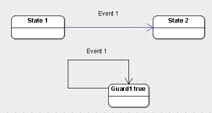
We start with a sample transition, as in the diagram.

Statemachine transition with guard

You move from State 1 to State 2 when Event 1 arrives, but only when guard() is true. Supposedly, guard() is a boolean expression on the World. It can be either true or false, or else we wouldn’t bother asking, and, supposedly, the World sometimes makes it true and sometimes makes it false. I’ll come back to this in a moment. Suppose, now, that, the World being in a state of making guard() true, is represented as a real state, in another statemachine.

Two automata

We now have two statemachines, and I’ve taken the liberty to make the World statemachine understand the Event 1 transition as well (not doing anything important with it). The reason I did that, was to pave the way to forming the intersection of the two statemachines.

Product of automata

What just happened, is that we got rid of the guard, at the cost of having to maintain a second statemachine, the World one. In a system where transitions in the World statemachine are also done from within the system itself, this amounts to optimizing the guard calculations to happen only when the World changes, and memoizing the result. The main statemachine should also understand (and similarly ignore) the events of the World one, so that the intersection statemachine is well-defined.

Don’t get all worked up about the complexity of all that, because you don’t have to physically form the intersection. All that “understanding” and “ignoring”, you should read it as happening implicitly. In plain words, you can just define transitions in the second machine in response to World-changing events, and transitions in the first machine in response to the main events, but the latter transitions will be defined on product-states, formed from one state from each statemachine.

I’ll be spending more time on statemachines in the immediate future, so you may expect more stuff coming from that direction. I can’t let you in on job-related things, but I’ll be happy to share basic knowledge.

Constraints on workflow paths, part 2

Continuing the effort to express constraints on workflow paths from the previous post, here is some practical advice for those who wish to undertake something similar, or simply retrace the same road.

First of all, I settled on SPOT. This was done for the following reasons: its on-line LTL-to-TGBA translator, as they call it, makes it easy to experiment; it can help you rephrase your LTL using automatic simplifications; it can output many different visual formats; its standalone executable can output standard LBTT; and, what I found quite helpful, it actually understands PSL in addition to LTL. PSL is a language “for specifying properties or assertions about hardware designs”. PSL supports SEREs (Sequential Extended Regular Expressions), which are formed like regular expressions, and can be combined with LTL expressions using special binding operators. Even though the whole expression can ultimately be expressed fully in plain LTL (and SPOT can formulate it that way for you), I found it easier to start with a SERE.

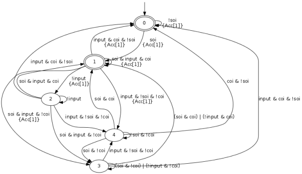
Which brings me to the formulation I arrived at for the property that troubled me in the end of the previous post: G(soi -> X(!input U (input & Fcoi))) (which SPOT can also output in fancy Unicode: □(○(¬input U (input∧◇coi))∨¬soi)). Its Büchi automaton is the following:

And here it is on the Web. Looks daunting, but you get used to it after a while. Let me show you how to produce it from the command line (Cygwin shell, in my case).

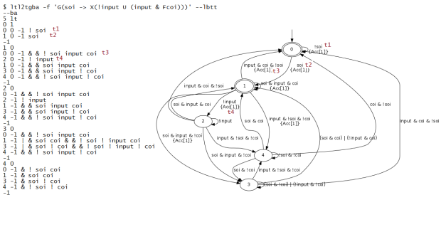
ltl2tgba -f 'G(soi -> X(!input U (input & Fcoi)))' --lbtt --ba

The LBTT output is the following.

4 2t
0 1
0 0 1 -1 ! soi
1 0 1 -1 soi
-1
1 0
0 0 1 -1 & & ! soi input coi
1 1 -1 ! input
1 0 1 -1 & & soi input coi
2 0 -1 & & soi input ! coi
3 0 -1 & & ! soi input ! coi
-1
2 0
0 0 1 -1 & & ! soi input coi
1 1 -1 & ! input coi
1 0 1 -1 & & soi input coi
2 -1 & ! input ! coi
2 0 -1 & & soi input ! coi
3 0 -1 & & ! soi input ! coi
-1
3 0
0 0 1 -1 & ! soi coi
1 0 1 -1 & soi coi
2 0 -1 & soi ! coi
3 0 -1 & ! soi ! coi
-1

To link the two, I have prepared an image where I link the first few transitions in the LBTT output to those on the automaton image.

You can take it from there…

The point of this exercise is the following: If you express your property in LTL and you’re prepared to jump through a few hoops, it is possible to invoke SPOT and read back a Büchi automaton for it, which you can use either to check your model, or as a run-time constraint checker. Now, there are ways to interface to SPOT so that you can provide your state space, as they call it, and SPOT will verify if the intersection of it with the automaton is empty or not. I have not explored it further. But using the resulting automaton as a generator for constraint-checking run-time infrastructure seems like what I wanted to do in Pandamator ever since I read about LTL.

I’m happy to close this post with a positive feeling! It’s not the end of the story, I promise you…

Constraints on workflow paths

I have mixed feelings about the current post. For the specific problem at hand, I had intended to develop a series of solutions, the one represented here being just the first one, soon to be replaced by a better one. However, for reasons I am going to go into later, I settled for this one, for the time being.

The domain of discourse is: workflow specifications, and how to verify them. Wide and under-specified enough to make for an interesting problem. My first thought for a quick-and-dirty solution, which would give some immediate results until the more elaborate ones brewed, was to develop a program to evaluate some pertinent constraints on possible paths through the workflow, and my choice for the language to use was Prolog. The reason is the painless facilities it has for state-space exploration: backtracking, incremental elaboration of data and pattern-matching through unification and conciseness. Plus, back in the ol’ days, I considered myself a decent Prolog programmer. Now, it could be debated whether tag “Esoteric” is really suitable for Prolog . After all, it has been around for more than forty years, and most universities teach it. However, it remains impenetrable for the uninitiated, and I don’t think many people actually learn it, even if they are taught about it.

For reasons unknown I had to start with Visual Prolog. Probably because I had avoided Turbo Prolog when it came out and I never had more than a casual glance at Mercury, Oz and other multi-paradigm languages.  That phase lasted the better part of two days, then I got fed up with the nagging message at startup and I went back to the less flashy SWI Prolog.To make a long story short, what I did was the following. My program loops through all of our workflows, reads them as Prolog facts and then runs the actual verification code on each one. The focus of this post is the actual verification code running on the graphs which encode the workflows.

Each verification rule looks for counter-examples of the property it encodes, which are paths through the graph. It consists of the following components: a selector of initial nodes, a filter that limits the edges taken from each node, and a selector of final nodes. Other than limiting the search space with the aid for those components, exploration is exhaustive, since we’re looking for counterexamples.

For example, the following clauses of the filter predicate for a particular rule, encode some workflow conditions on having or not having passed through a prior workflow step (and the lack of syntax highlighting for Prolog from WordPress certainly justifies the “Esoteric” tag).

allowed_arc(N,V) :-
	stepcond(N,through(I)),
	member(I,V),
	!.
allowed_arc(N,V) :-
	stepcond(N,not_through(I)),
	member(I,V),
	!, fail.

As you can see, the filtering predicate takes as parameters the node to go to, and the sequence of previously visited nodes. The filtering predicated is called by predicate possible_path, which computes the path.

possible_next(V, Pr, X, Y) :-
	stepact(X,goto(Y)),
	apply(Pr,[Y,V]).
possible_next(V, Pr, X, Y) :-
	stepcond(Y,input(_)),
	X \= Y,
	apply(Pr,[Y,V]).

possible_path(V,_,X,X,P) :-
	reverse(V,P).
possible_path(V, Pr, X, Z, P) :-
	possible_next(V,Pr,X,Y),
	possible_path([Y|V],Pr,Y,Z,P).

Evaluating the rule is done with the help of findall.

findall(
	P,
	(stepact(F,soi),
		possible_path([F],allowed_arc,F,Z,P),
		length(P,L),
		L > 1,
		stepact(Z,soi)),
	X4)

It needs a second look, so let me break it up.

stepact(F,soi) Start from every action matching the particular fact pattern.

possible_path([F],allowed_arc,F,Z,P) Enumerate all possible paths using the particular filter.

length(P,L), L > 1, stepact(Z,soi) Stop for all paths of length > 1 whose final node matches the particular fact pattern.

A brute-force solution, but managed to sniff out several potential problems in the workflows and has room to grow with new rules. Why did I say that its only purpose was to pave the way for more elaborate solutions?

My hope was to use formal verification methods, and I had every reason to be hopeful because I had multiple candidates to try.

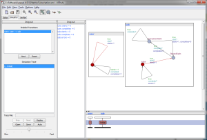
The first one was UPPAAL, a tool which allows one to specify timed automata, simulate them and verify invariants expressed in CTL. Sounds cool, doesn’t it?

The problem is, encoding your system in this way is not an easy task, and probably not something that could be done by translating a workflow specification automatically. And people who used it independently had trouble adapting the tool to their problem and ended up actually playing to the strengths of the tool. It’s not out the question, but it needs a lot of time and dedication, and it is not a short-term study.

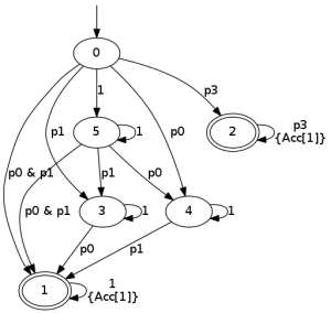
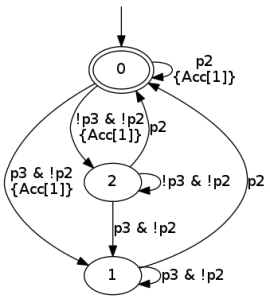
My other hope was to express the path constraints using LTL, instead of the unstructured way I was using. Which necessitated a lot of research to find how LTL can be verified and what tools there are to aid one in this endeavor. It turns out there are, and some of them have been also put online for people to test! Try out LTL2BA and SPOT. And, if you persevere through various tortures imposed on you by the intricacies of cross-platform C/C++ builds, you can actually find yourself with real singing and dancing LTL2BA and SPOT executables that you can invoke. Best of all, they can both be made to output (semi-?) standard LBT format. To give you an idea, the formula G p3 | (F p0 & F p1) results in the following Büchi automaton (yes, that’s what it’s called) which can be used to verify it at run-time.

This was something I’ve been considering for Pandamator, as well, to express constraints for whole object lifetimes. As I found out, it was not a novel idea, but maybe I’d have the honor of implementing it first in an accessible way. It would need some elaborate machinery: abstract away all logic that is not LTL (formulas to translate have simple propositional variables), invoke an external program, read back the automaton and fill back in the actual logic conditions. That would replace my hodge-podge filters and selectors with something having real logical backing. The problem is, trying to write the darned LTL constraints proved to be not evident!

For example, how would the following be written? After action p0, action p2 cannot appear unless condition p1 appears between them. My guess would be p0 -> X G ((!p1 & !p2) U (p1 U p2)). However, the automaton does not seem to be suitable.

This is my current situation… Maybe an intermediate solution would be to formulate an automaton directly, and use it as the specification of the constraint.

I won’t pretend I know the answer. I’m in the dark, but I’m determined to see this through. And, in the meantime, my lowly Prolog program can actually chug along and produce useful results…

Strong Typing? It’s not really strong enough…

Maybe it’s just age, but I find myself slipping into being less and less tolerant of weak type-systems. Which may come as a surprise, given my involvement in TinyScheme, but I don’t see it as a contradiction. Scripting is a different kind of work than writing multi-module, complicated software, and it’s nice to be able to use a language that can express the Y combinator for the former. For the latter, though, I am becoming more and more autocratic. I want to deprive my programs from all freedom to do as they please. I frown when I see mission-critical software written in Python. I turn away when I see customer-facing software written in Perl. And I growl when I see big programs written in PHP. I’d lose sleep if I thought there were a place in my code ready to do something silly when I least expect it, “silly” being a synonym for “something a typechecker would catch right away”. And I’m not talking about preconditions, postconditions and assertions, because these will still take action at run-time. Although Bertrand Meyer’s Eiffel bringing them forth was very revolutionary, twenty-so years ago, given that they are not mainstream concepts even now. What I’m talking about, is incorporating more programmer intent into the type-system proper.

I want to introduce you to F* (F-Star) which you will find familiar-looking if you’re coming from F# (if you’re coming from Haskell, have a look at Agda, which covers similar ground). You can play with it on Rise4Fun through a simple browser without going into the trouble of installing anything. If you’re into .Net in general, have a look at Code Contracts, they are now being incorporated into the development ecosystem, so maybe they’ll become mainstream. It uses the same verification engine as F* (Z3), and it’s available right now (it has Code Contracts examples on Rise4Fun, as well). But I’m going to follow the F*/Agda direction in this post.

F* adds types of types (called kinds), so type constructors are typed (kinded) themselves. For example, “list” is actually a type constructor of kind * => *.

type list :: * => * =
   | Nil : 'a::* -> list 'a
   | Cons : 'a::* -> 'a -> list 'a -> list 'a

This is just a new point of view on usual functional notions. Here comes a new thing: term-indexed (or dependent) types. The following type is the length-indexed list, of kind int => * => *, meaning that it constructs a *-kinded type from an int-typed term and a *-kinded type.

type ilist :: int => * => * =
   | INil  : ilist 0 'a
   | ICons : x:'a -> n:int -> ilist n 'a -> ilist (n + 1) 'a

The real fun begins when you create functions of dependent types, like the following function to append two length-indexed lists (the Rise4Fun tutorial has these examples and more).

val iappend: n1:int -> ilist n1 'a -> n2:int -> ilist n2 'a -> ilist (n1 + n2) 'a
let rec iappend n1 l1 n2 l2 = match l1 with
   | INil -> l2
   | ICons x n1_minus_1 l1tl ->
     ICons x (n1_minus_1 + n2) (iappend n1_minus_1 l1tl n2 l2)

Something more is evident in the function signature, compared to that of a usual appending function. You can actually read, in the signature, the constraint that the length of the list this function produces is the sum of the lengths of its two list arguments. This is just a minimal example, and I’m afraid the full power of term-indexed types will not be evident to you from the F* tutorial alone. Material on Agda has more pointers to how on can embed propositional logic in dependent types. I hope you’re as excited as me with this prospect, which could sort-of merge what declarative constraints (like those on Code Contracts) can be expressed in the type-system itself, and functions will actually prove that what they’re doing has the intended properties, purely by doing type-correct operations!

Please go and play with the F* tutorial. It will not help you in your everyday job (but if you do have a job where F* can help you, please be kind enough to not tell me…), but it will open your mind to things that will come. When I was reading the Gentle Introduction to Haskell twenty years ago, I did not know that I’d be actually using F# and closures in C# twenty years hence.

But be prepared for a rough ride, because you won’t have the support you enjoy in the mainstream. For example, while trying to write the following function to map a length-indexed list to another, I stumbled on type errors, which, of course, is the idea.

val imap: n:int -> ('a -> 'b) -> ilist n 'a -> ilist n 'b
let rec imap (n:int) (f:'a->'b) (l1:ilist n 'a) = match l1 with
   | INil -> INil
   | ICons x n1 l1tl -> ICons (f x) n1 (imap n1 f l1tl)

Even so, getting errors like the following is not really helpful.

input(13,45-14,0) : Error : Expected an expression of type:

ILIST1.ilist x_11_2 'x_10_1

but got (x_13_2): ILIST1.ilist x_13_1 'x_10_1

Type checking failed: ILIST1

Well, that’s why it’s called the “bleeding edge”…

APL, J, NIAL and Array Theory

When I was in France, I was doing a stage with Jean-Louis Laurière in a company that dealt with payroll software and services. The idea was to express all payroll logic in a rule-based system, and he had enrolled a senior person, very knowledgeable on the subject, to explain some aspect of it over lunch. That person was a very experienced COBOL programmer and, at one point, after he had explained some calculation using nested loops, I tried to summarize:

– So, this is the Min of x and the Max of y and z.

I got a blank stare and later, when we were alone with Jean-Louis, he said he almost burst into laughter at that moment, because it was obvious he did not understand what I was saying. Mind you, he knew perfectly well how to calculate the number in question procedurally, but he lacked the concepts to express it in the succinct way I was using. He was using a lower level of abstraction, and, since there seems to be a limit on the “chunks” we can hold in our heads, the higher the level of abstraction we use, the further away our minds can reach.

Those of you that share my fascination with Functional Programming probably like it for the same reason: you can express so darned more if you use a higher level of abstraction (higher order functions, in this case). All the better, if modern implementations can perform so well that you can use this abstraction for real-life computations. This post is not about Functional Programming. There are zillion sources to read about that. This post is about what higher abstractions might look like on the realm of array programming and, in particular, APL-like languages. In another post, I might write about the three languages that contested for the HPCS.

One thing you should understand while reading about those languages is that the APL branch of languages spawed away from the conventional trunk very early. I have found a copy of “A Programming Language” and I guess that a Fortran programmer reading it at the time must have felt like someone having found the manual for the Flux Capacitor in the Middle Ages. It’s a safe guess, because I can safely imagine a Java programmer of today feeling the same, since the concepts it is based on are as much distant from Java as they are from Fortran. In fact, the Fortran programmer probably has an edge, since Fortran is ultimately concerned with manipulating array data in the first place. I hope I have tickled your fancy enough to spend some time researching APL, but I’m going to propose an easier route: study J instead, which has a free implementation, can be written in ASCII (you must surely be wondering what APL is written in, if not ASCII) and you can find a very good introductory text from the conventional viewpoint: “J for C Programmers” (can be found in the J Books). This book is very important for the outsider, because it appears that all other sources present J like the most natural thing on earth which only your limited brainpower perceives as different. Sorry, no “J for Functional Programmers” exists, but this is no big deal as array programming has no different treatment in functional languages that in conventional ones. Although you will surely have little voices in your mind whispering about higher order functions while you’ll be reading about J adverbs. Curiously, a presentation of array programming that seems more close to the language of the functional programmer can be found in material for NIAL (download Papers.zip and don’t go to the root of the site), which I did not know but read about in the APL F.A.Q. Array Theory seems like a good theoretical underpinning for such languages.

Rule #34 of the internet supposedly says that, if something exists, there’s porn for it. Here’s some J porn for you. I used this as a programming test once believing that, someone who can learn enough J to answer this, can learn anything else needed on the job. I was not let down.

Given a 9×9 array of integers from 1 to 9, forming the supposed solution to a Sudoku puzzle (http://en.wikipedia.org/wiki/Sudoku), write a J verb (program) that computes whether the 9×9 array is, indeed, a solution according the following rules for Sudoku: Every line, every row and every 3×3 tile (3×3 tiles are arranged in a 3×3 arrangement to tile the entire array, see Wikipedia article) should contain every number from 1 to 9 one unique time.

The solution should use verb ranks to partition the array in all the needed ways (cells), and determine uniqueness by applying the same test verb in the appropriate manner.

And this is my own solution to that.

test3 =: monad define
                items =. ,y
                (9=#~.items) *. *./(items>0),(items<10)
)

is_sudoku3 =: monad define
                *./ (test3"_1 y) , (test3"_1 |: y) , (,(3 3 ,: 3 3) test3;._3 y)
)

Update: At the time I devised this exercise I could not find any relevant article, but I just now found a full Sudoku solver in J at the J Wiki.